Probability theory is a branch of mathematics that deals with the study of uncertainty and randomness. It provides a framework for quantifying and reasoning about uncertainty, allowing us to model and analyze various phenomena that involve chance or randomness. The central concept in probability theory is the probability, which represents the likelihood of different outcomes in a random experiment.
tibble [344 × 8] (S3: tbl_df/tbl/data.frame)
 $ species          : Factor w/ 3 levels "Adelie","Chinstrap",..: 1 1 1 1 1 1 1 1 1 1 ...
 $ island           : Factor w/ 3 levels "Biscoe","Dream",..: 3 3 3 3 3 3 3 3 3 3 ...
 $ bill_length_mm   : num [1:344] 39.1 39.5 40.3 NA 36.7 39.3 38.9 39.2 34.1 42 ...
 $ bill_depth_mm    : num [1:344] 18.7 17.4 18 NA 19.3 20.6 17.8 19.6 18.1 20.2 ...
 $ flipper_length_mm: int [1:344] 181 186 195 NA 193 190 181 195 193 190 ...
 $ body_mass_g      : int [1:344] 3750 3800 3250 NA 3450 3650 3625 4675 3475 4250 ...
 $ sex              : Factor w/ 2 levels "female","male": 2 1 1 NA 1 2 1 2 NA NA ...
 $ year             : int [1:344] 2007 2007 2007 2007 2007 2007 2007 2007 2007 2007 ...
summary(penguins)
      species          island    bill_length_mm  bill_depth_mm
 Adelie   :152   Biscoe   :168   Min.   :32.10   Min.   :13.10
 Chinstrap: 68   Dream    :124   1st Qu.:39.23   1st Qu.:15.60
 Gentoo   :124   Torgersen: 52   Median :44.45   Median :17.30
                                 Mean   :43.92   Mean   :17.15
                                 3rd Qu.:48.50   3rd Qu.:18.70
                                 Max.   :59.60   Max.   :21.50
                                 NA's   :2       NA's   :2
 flipper_length_mm  body_mass_g       sex           year
 Min.   :172.0     Min.   :2700   female:165   Min.   :2007
 1st Qu.:190.0     1st Qu.:3550   male  :168   1st Qu.:2007
 Median :197.0     Median :4050   NA's  : 11   Median :2008
 Mean   :200.9     Mean   :4202                Mean   :2008
 3rd Qu.:213.0     3rd Qu.:4750                3rd Qu.:2009
 Max.   :231.0     Max.   :6300                Max.   :2009
 NA's   :2         NA's   :2
   Min. 1st Qu.  Median    Mean 3rd Qu.    Max.
  172.0   190.0   197.0   200.9   213.0   231.0
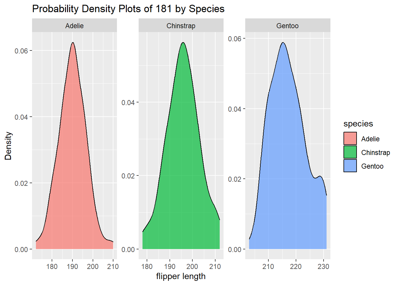
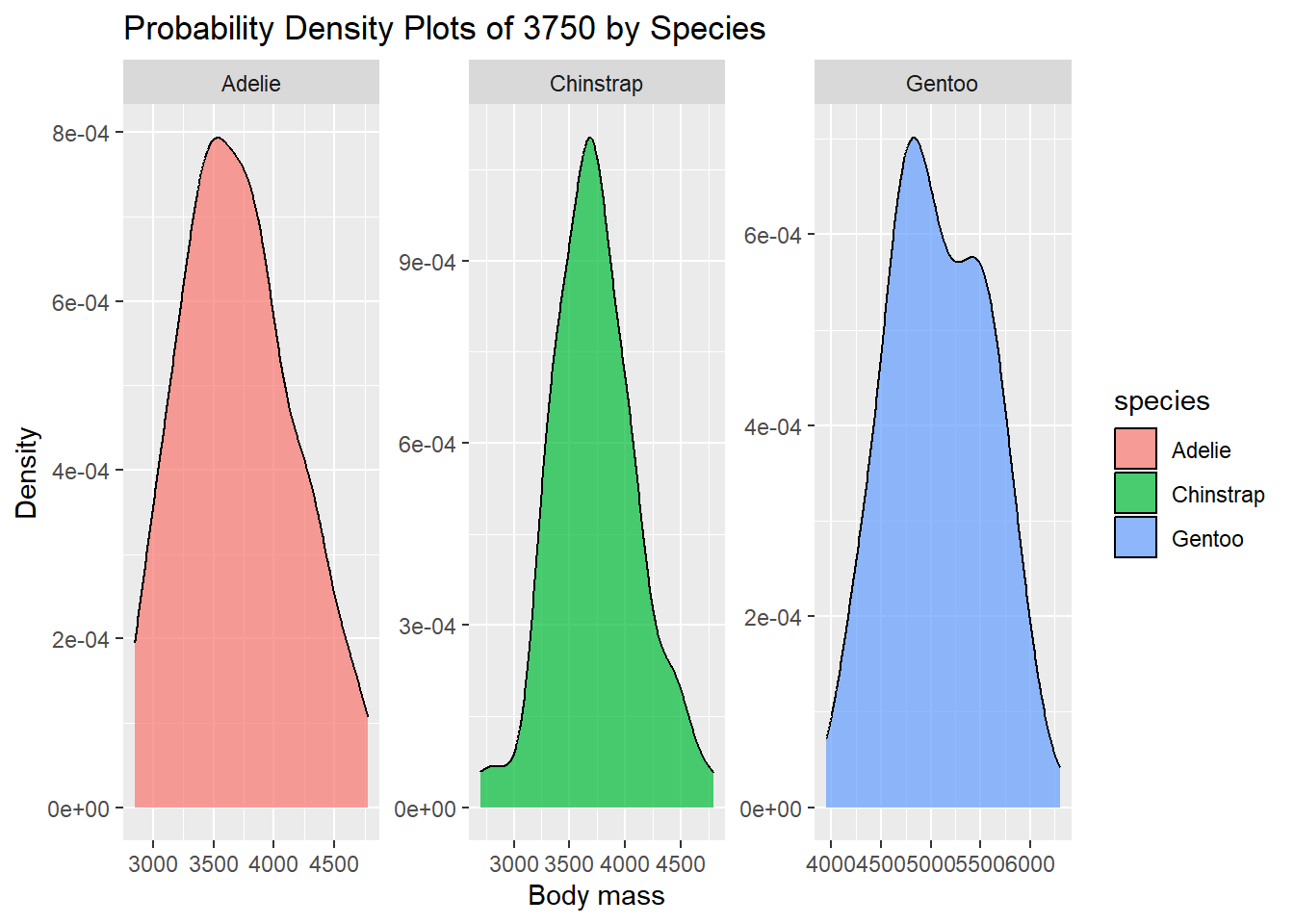
# Select one continuous variables for probability density plotsselected_vars <-c(penguins$flipper_length_mm)selected_vars2 <-c(penguins$bill_length_mm) selected_vars3 <-c(penguins$body_mass_g) # Create probability density plots for each variable by speciespenguin_density_plots <-ggplot(penguins, aes(x = selected_vars, fill = species)) +geom_density(alpha =0.7) +facet_wrap(~species, scales ="free") +labs(title =paste("Probability Density Plots of", selected_vars, "by Species"), x ="flipper length", y ="Density")print(penguin_density_plots)
penguin_density_plots2 <-ggplot(penguins, aes(x = selected_vars2, fill = species)) +geom_density(alpha =0.7) +facet_wrap(~species, scales ="free") +labs(title =paste("Probability Density Plots of", selected_vars2, "by Species"), x ="bill length", y ="Density")print(penguin_density_plots2)
#conditional probabilities# Create a contingency table for species and islandcontingency_table_island <-table(penguins$species, penguins$island)# Calculate conditional probabilities given the islandconditional_probabilities_island <-prop.table(contingency_table_island, margin =1)# Create a contingency table for species and sexcontingency_table_sex <-table(penguins$species, penguins$sex)# Calculate conditional probabilities given the sexconditional_probabilities_sex <-prop.table(contingency_table_sex, margin =1)# Print the contingency tablesprint("Contingency Table for Species and Island:")
A random variable is a mathematical function that assigns a numerical value to each outcome in the sample space of a random experiment. It serves as a way to quantify and analyze the variability and uncertainty associated with random processes. Random variables can be classified as either discrete or continuous.
# Simulate rolling a fair six-sided diedie_outcomes <-1:6# Define random variables X and YX <-sample(die_outcomes, 1, replace =TRUE)Y <-sample(die_outcomes, 1, replace =TRUE)# Print the outcomes of X and Ycat("Outcome of X:", X, "\n")
Outcome of X: 5
cat("Outcome of Y:", Y, "\n")
Outcome of Y: 2
# Calculate the sum ZZ <- X + Ycat("Sum Z:", Z, "\n")
Sum Z: 7
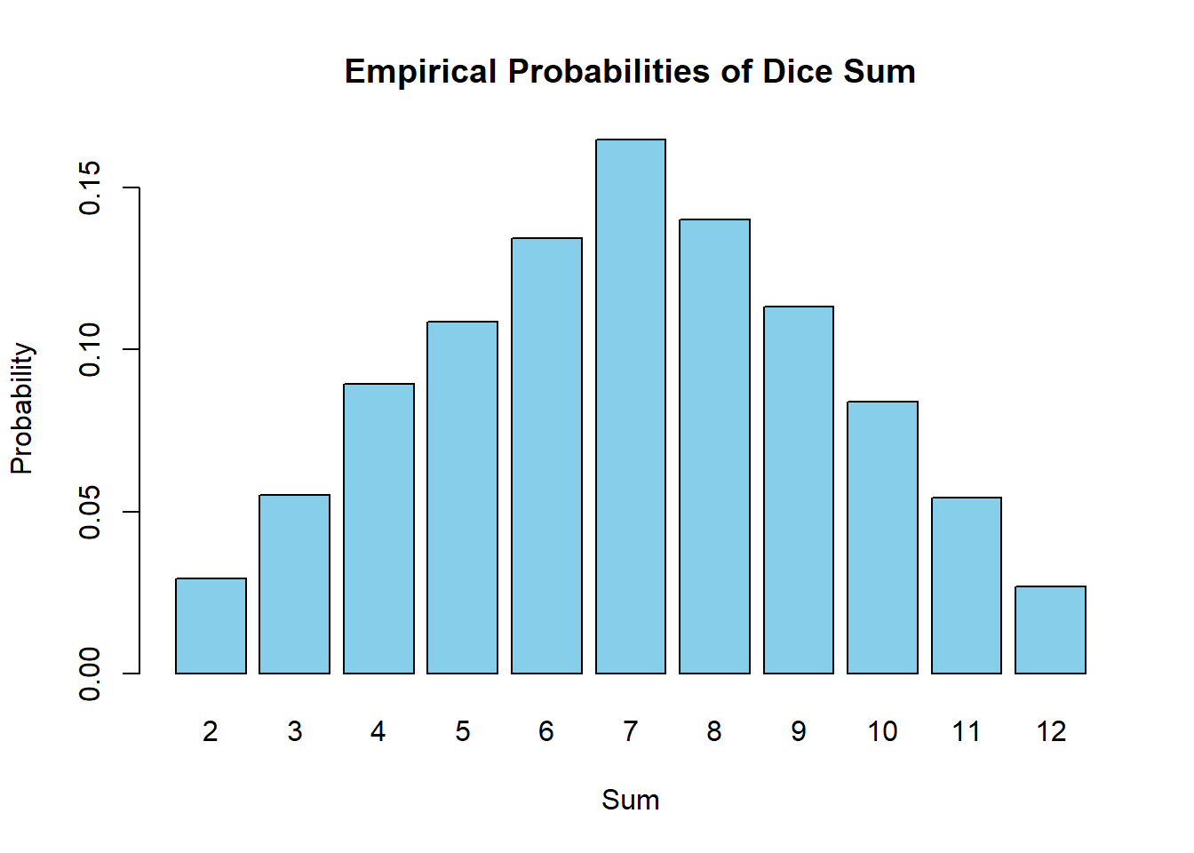
# Simulate rolling the dice multiple times to estimate probabilitiesnum_simulations <-10000# Simulate X and Ysimulated_X <-sample(die_outcomes, num_simulations, replace =TRUE)simulated_Y <-sample(die_outcomes, num_simulations, replace =TRUE)# Calculate the sum Z for each simulationsimulated_Z <- simulated_X + simulated_Y# Calculate the empirical probabilitiesempirical_probabilities <-table(simulated_Z) / num_simulations# Print the empirical probabilitiescat("Empirical Probabilities for Z:\n")
# Plot the empirical probabilitiesbarplot(empirical_probabilities, names.arg =2:12, col ="skyblue", main ="Empirical Probabilities of Dice Sum", xlab ="Sum", ylab ="Probability")