Regression

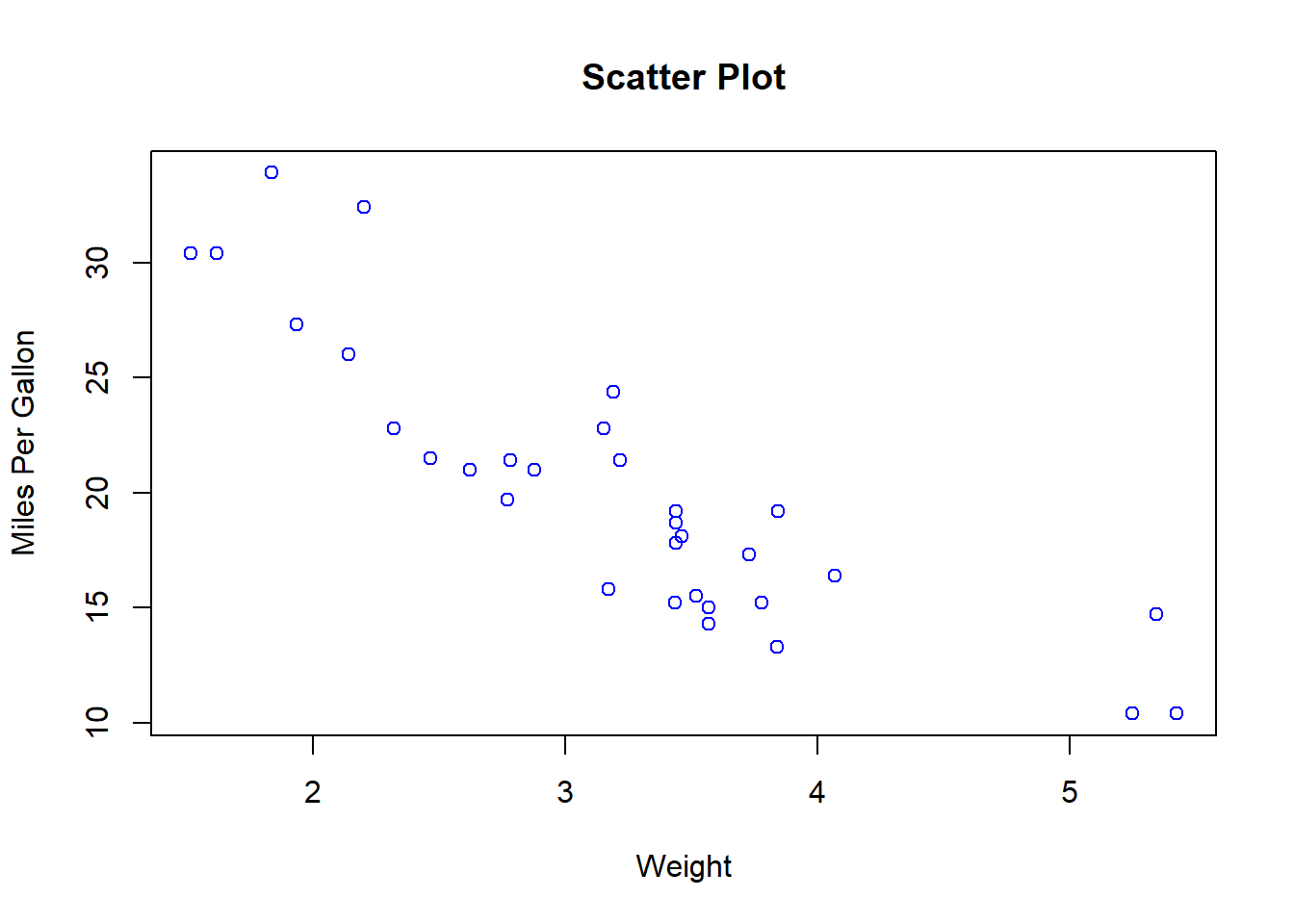
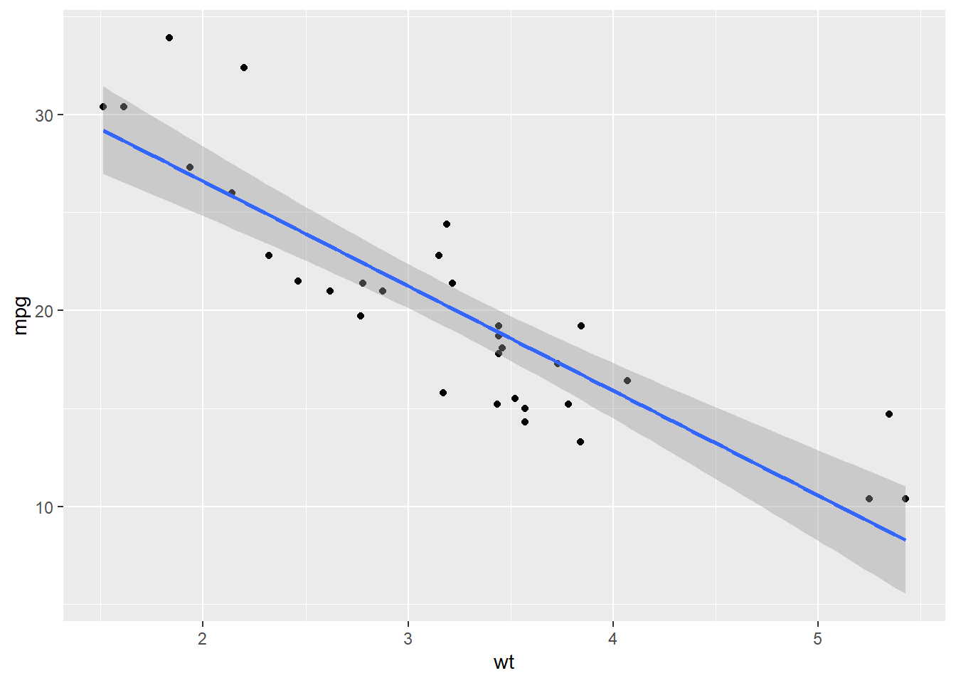
In this blog, we’ll use the GLM to perform simple linear regression. Below,you will find me using mtcars data for fitting a linear regression model between the variables weight and miles per gallon for car dataset.

1. Simple linear regression

• Definition: Simple linear regression involves predicting a dependent variable (response) based on a single independent variable (predictor).

• Equation: y=β0+β1x+ϵ, where y is the dependent variable, x is the independent variable, β0​ is the intercept, β1​ is the slope, and ϵ is the error term

library(ggplot2)

# Load the mtcars dataset
data(mtcars)

# Explore the dataset
head(mtcars)

                   mpg cyl disp  hp drat    wt  qsec vs am gear carb
Mazda RX4         21.0   6  160 110 3.90 2.620 16.46  0  1    4    4
Mazda RX4 Wag     21.0   6  160 110 3.90 2.875 17.02  0  1    4    4
Datsun 710        22.8   4  108  93 3.85 2.320 18.61  1  1    4    1
Hornet 4 Drive    21.4   6  258 110 3.08 3.215 19.44  1  0    3    1
Hornet Sportabout 18.7   8  360 175 3.15 3.440 17.02  0  0    3    2
Valiant           18.1   6  225 105 2.76 3.460 20.22  1  0    3    1

summary(mtcars)

      mpg             cyl             disp             hp       
 Min.   :10.40   Min.   :4.000   Min.   : 71.1   Min.   : 52.0  
 1st Qu.:15.43   1st Qu.:4.000   1st Qu.:120.8   1st Qu.: 96.5  
 Median :19.20   Median :6.000   Median :196.3   Median :123.0  
 Mean   :20.09   Mean   :6.188   Mean   :230.7   Mean   :146.7  
 3rd Qu.:22.80   3rd Qu.:8.000   3rd Qu.:326.0   3rd Qu.:180.0  
 Max.   :33.90   Max.   :8.000   Max.   :472.0   Max.   :335.0  
      drat             wt             qsec             vs        
 Min.   :2.760   Min.   :1.513   Min.   :14.50   Min.   :0.0000  
 1st Qu.:3.080   1st Qu.:2.581   1st Qu.:16.89   1st Qu.:0.0000  
 Median :3.695   Median :3.325   Median :17.71   Median :0.0000  
 Mean   :3.597   Mean   :3.217   Mean   :17.85   Mean   :0.4375  
 3rd Qu.:3.920   3rd Qu.:3.610   3rd Qu.:18.90   3rd Qu.:1.0000  
 Max.   :4.930   Max.   :5.424   Max.   :22.90   Max.   :1.0000  
       am              gear            carb      
 Min.   :0.0000   Min.   :3.000   Min.   :1.000  
 1st Qu.:0.0000   1st Qu.:3.000   1st Qu.:2.000  
 Median :0.0000   Median :4.000   Median :2.000  
 Mean   :0.4062   Mean   :3.688   Mean   :2.812  
 3rd Qu.:1.0000   3rd Qu.:4.000   3rd Qu.:4.000  
 Max.   :1.0000   Max.   :5.000   Max.   :8.000  

# Scatter plot
plot(mtcars$wt, mtcars$mpg, main="Scatter Plot", xlab="Weight", ylab="Miles Per Gallon", col="blue")

# Fit the linear regression model
model <- lm(mpg ~ wt, data = mtcars)

# Display the summary of the model
summary(model)

Call:
lm(formula = mpg ~ wt, data = mtcars)

Residuals:
    Min      1Q  Median      3Q     Max 
-4.5432 -2.3647 -0.1252  1.4096  6.8727 

Coefficients:
            Estimate Std. Error t value Pr(>|t|)    
(Intercept)  37.2851     1.8776  19.858  < 2e-16 ***
wt           -5.3445     0.5591  -9.559 1.29e-10 ***
---
Signif. codes:  0 '***' 0.001 '**' 0.01 '*' 0.05 '.' 0.1 ' ' 1

Residual standard error: 3.046 on 30 degrees of freedom
Multiple R-squared:  0.7528,    Adjusted R-squared:  0.7446 
F-statistic: 91.38 on 1 and 30 DF,  p-value: 1.294e-10

# Visualize the regression line


ggplot(mtcars, aes(wt, mpg)) +
  geom_point() +
  stat_smooth(method = lm)

`geom_smooth()` using formula = 'y ~ x'

2. Non-Linear Regression Models:

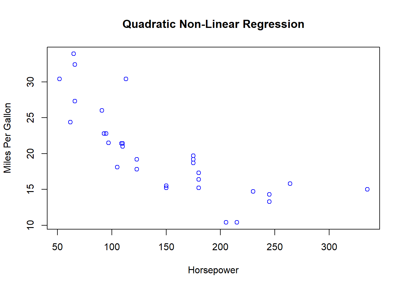
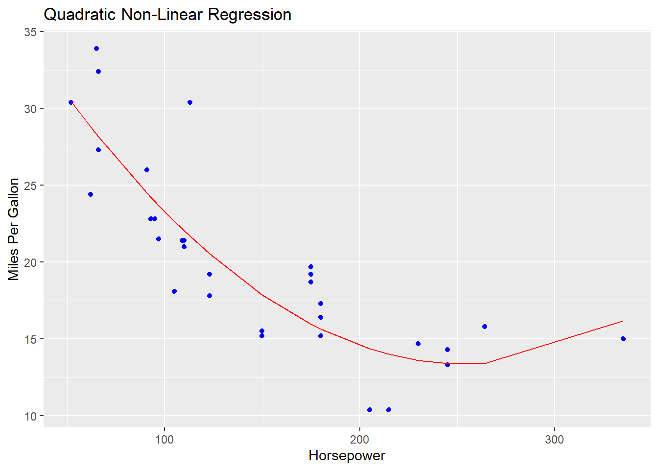
Linear regression models assume a linear relationship between the independent variables and the dependent variable. However, in many real-world scenarios, the relationship may not be strictly linear. Non-linear regression models are used when the relationship between variables is better described by a non-linear equation.

# Load the mtcars dataset
data(mtcars)

# Fit a quadratic non-linear regression model
model <- lm(mpg ~ poly(hp, 2), data = mtcars)

# Generate predicted values
predictions <- predict(model, newdata = data.frame(hp = mtcars$hp))

# Plot the data and non-linear regression curve
plot(mtcars$hp, mtcars$mpg, main="Quadratic Non-Linear Regression", xlab="Horsepower", ylab="Miles Per Gallon", col="blue")

ggplot(mtcars, aes(x = hp, y = mpg)) +
  geom_point(color = "blue") +
  
  # Add a dashed line for the non-linear regression curve
  geom_line(aes(y = predictions), color = "red") +
   # Labels and title
  labs(title = "Quadratic Non-Linear Regression",
       x = "Horsepower",
       y = "Miles Per Gallon") 

# Display the model summary
summary(model)

Call:
lm(formula = mpg ~ poly(hp, 2), data = mtcars)

Residuals:
    Min      1Q  Median      3Q     Max 
-4.5512 -1.6027 -0.6977  1.5509  8.7213 

Coefficients:
             Estimate Std. Error t value Pr(>|t|)    
(Intercept)    20.091      0.544  36.931  < 2e-16 ***
poly(hp, 2)1  -26.046      3.077  -8.464 2.51e-09 ***
poly(hp, 2)2   13.155      3.077   4.275 0.000189 ***
---
Signif. codes:  0 '***' 0.001 '**' 0.01 '*' 0.05 '.' 0.1 ' ' 1

Residual standard error: 3.077 on 29 degrees of freedom
Multiple R-squared:  0.7561,    Adjusted R-squared:  0.7393 
F-statistic: 44.95 on 2 and 29 DF,  p-value: 1.301e-09